Section Week 1

This is an outline of the topics we covered in the first week of class. These notes are not a substitute for your own note-taking. I highly recommend that you take your own notes during class. If you ever miss a class for any reason, reach out to another student in class to get a copy of their notes.

Subsection Tuesday 1/13

Subsubsection Sec 1.1: Sets

In prior math courses, you mostly asked deterministic questions. Now, we need new tools to model randomness.
Example 1.
A toxin molecule in a cell has a certain chance each minute to leave the cell.
Example 2.
A patient takes a diagnostic test for a disease and wants to know the chance that they have the disease based on the test result.
Definition 3.
The sample space, often denoted \(\Omega\text{,}\) is the set of all possible results of an experiment. A single result is called an outcome, while a collection of results is called an event.
Example 4.
An experiment consists of rolling a standard 6-sided die (D6). The sample space is \(\Omega = \{1, 2, 3, 4, 5, 6\}\text{.}\) One possible event is \(A = \{2, 4, 6\}\text{,}\) i.e., the event that the result of the roll is even.
Note: we’ll use notation like D6 to indicate a 6-sided die with faces 1, 2, 3, 4, 5, 6. Similarly, for example, D4 will indicate a 4-sided die with faces 1, 2, 3, 4.
Definition 5.
The symbol \(\in\) means "is an element of", as in \(4 \in A\text{.}\)
The symbol \(\subset\) means "is a subset of", as in \(A \subset \Omega\text{.}\) This means that every element of the set \(A\) is also an element of the set \(\Omega\text{.}\)
Definition 6.
Consider sets \(A\) and \(B\text{,}\) each contained inside \(\Omega\text{.}\) We can combine sets in a variety of ways:
Union
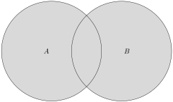
The union of \(A\) and \(B\) is the set \(A \cup B = \{x \mid x \in A \text{ or } x \in B\}\text{.}\)
Intersection
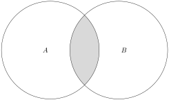
The intersection of \(A\) and \(B\) is the set \(A \cap B = \{x \mid x \in A \text{ and } x \in B\}\text{.}\)
Difference
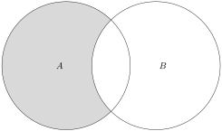
The set difference \(A-B\) is the set \(A - B = \{x \mid x \in A \text{ and } x \notin B\}\text{.}\)
Complement
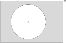
The complement of \(A\) is the set \(A^c = \{x \in \Omega \mid x \notin A\}\text{.}\)
Empty Set
The empty set, usually written \(\emptyset\) or \(\{\}\text{,}\) is the set which contains no elements.
It’s useful sometimes to draw pictures called Venn diagrams representing set interactions.
described in detail following the image
Venn diagram showing sets \(A, B\) with the region representing \(A \cup B\) shaded.
Figure 7. Union
described in detail following the image
Venn diagram showing sets \(A, B\) with the region representing \(A \cap B\) shaded.
Figure 8. Intersection
described in detail following the image
Venn diagram showing sets \(A, B\) with the region representing \(A - B\) shaded.
Figure 9. Difference
described in detail following the image
Venn diagram showing set \(A \subset \Omega\) with the region representing \(A^c\) shaded.
Figure 10. Complement

Subsubsection Sec 1.2: Probability

Next, we want to start assigning probabilities to each individual outcome so we can then find the probabilities of events.
Example 11.
An experiment consists of rolling a D6. The sample space is \(\Omega = \{1, 2, 3, 4, 5, 6\}\text{.}\) We might assign probabilities as follows:
Table 12. Distribution for a fair die
\(x\) \(\Pr(x)\)
1 \(1/6\)
2 \(1/6\)
3 \(1/6\)
4 \(1/6\)
5 \(1/6\)
6 \(1/6\)
Note that we don’t have to assign the same probability to each outcome. If we do, we call this distribution uniform. If we have some event, such as \(A = \{2, 4, 6\}\text{,}\) then we calculate the probability of the event by adding together the probabilities of the outcomes that make up the event:
\begin{gather*} \Pr(A) = \Pr(2) + \Pr(4) + \Pr(6) = \frac{1}{6} + \frac{1}{6} + \frac{1}{6} = \frac{3}{6} = \frac{1}{2} \end{gather*}
Note that this is the same result that we would get if we counted the total number of outcomes in \(A\) and divided by the total number of outcomes in \(\Omega\text{.}\)
Definition 13.
Given a finite set \(A\text{,}\) the cardinality of \(A\text{,}\) written \(|A|\text{,}\) is the number of elements in \(A\text{.}\)
Example 15.
Suppose we have a weighted die that’s much more likely to come up 6 than any other outcome.
Table 16. Distribution for a fair die
\(x\) \(\Pr(x)\)
1 0.1
2 0.1
3 0.1
4 0.2
5 0.1
6 0.4
With this distribution, if \(A = \{2, 4, 6\}\text{,}\) then:
\begin{gather*} \Pr(A) = 0.1 + 0.2 + 0.4 = 0.7 \neq \frac{3}{6}. \end{gather*}
Example 17.
Pick a number from 1 to 10. What is the probability of picking 3?
Some considerations:
  1. Are we using the uniform distribution?
  2. What even is the sample space here? Do we need to pick only integers, or is \(\pi\) an outcome here?
  3. What would "uniform" mean if the sample space was infinite?
Definition 18.
A probability distribution on a sample space \(\Omega\) assigns probabilities to every event, satisfying the following conditions:
  1. \(\Pr(\Omega) = 1\text{.}\)
  2. \(0 \leq \Pr(A) \leq 1\) for any event \(A\text{.}\)
  3. If \(A \cap B = \emptyset\text{,}\) then \(\Pr(A\cup B) = \Pr(A) + \Pr(B)\text{.}\)
Example 19.
Suppose we flip a coin until we see heads. The sample space is \(\Omega = \{H, TH, TTH, TTTH, \dotsc\}\text{.}\) What would "uniform" mean here? Is there any way we could assign the same probability to each individual outcome here?
Instead of "uniform", what if we want to treat the coin as a fair coin? Then what would the distribution be?
Table 20. Distribution assuming a fair coin
\(x\) # flips \(\Pr(x)\)
\(H\) 1 \(1/2\)
\(TH\) 2 \(1/4\)
\(TTH\) 3 \(1/8\)
\(TTTH\) 4 \(1/16\)
\(\vdots\) \(\vdots\)
\(T\dotsm TH\) \(n\) \(1/2^n\)
\(\vdots\) \(\vdots\)
Example 21.
One last (very useful!) observation. Recall: If \(A\cap B = \emptyset\text{,}\) then \(\Pr(A\cup B) = \Pr(A) + \Pr(B)\text{.}\)
For any event \(A\text{,}\) \(A\cap A^c = \emptyset\) and \(A \cup A^c = \Omega\text{.}\) So:
\begin{gather*} 1 = \Pr(\underbrace{A \cup A^c}_{\Omega}) = \Pr(A) + \Pr(A^c). \end{gather*}
We can rewrite this in two useful ways:
\begin{align*} \Pr(A) \amp = 1 - \Pr(A^c) \\ \Pr(A^c) \amp = 1 - \Pr(A) \end{align*}

Subsection Thursday 1/15

Subsubsection Conditional Probability

Question: How does evidence (e.g., knowledge of one event occurring) change our knowledge of probabilities for other events?
Example 22.
Roll a fair D6 two times. Let \(A = \{\text{sum } \geq 10\}\) and \(B = \{\text{first roll is } 6\}\text{.}\) \(A\) feels more likely if we already know \(B\) has occurred.
Definition 23.
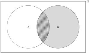
The conditional probability of \(A\) given \(B\) is: ,
\begin{gather*} \Pr(A \mid B) = \frac{\Pr(A\cap B)}{\Pr(B)} \end{gather*}
described in detail following the image
Two overlapping circles representing events \(A\) and \(B\) sit inside a rectangle representing the sample space \(\Omega\text{.}\) The circle labeled \(B\) is shaded. The portion of that circle which is overlapped by the \(A\) circle is also filled in with slanted lines.
Figure 24. \(\Pr(A \mid B)\) tells the proportion of \(B\) which is overlapped by \(A\text{.}\)
Example 25.
Continuing from the previous example, \(|\Omega| = 36\text{.}\)
\begin{align*} A \amp = \{(4, 6), (5, 5), (5, 6), (6, 4), (6, 5), (6, 6)\} \\ B \amp = \{(6, 1), (6, 2), (6, 3), (6, 4), (6, 5), (6, 6)\} \\ A \cap B \amp = \{(6, 4), (6, 5), (6, 6)\} \end{align*}
So \(\Pr(A) = \frac{6}{36}, \Pr(B) = \frac{6}{36}, \text{and } \Pr(A\cap B) = \frac{3}{36}\text{.}\) Then:
\begin{gather*} \Pr(A \mid B) = \frac{\Pr(A\cap B)}{\Pr(B)} = \frac{3/36}{6/36} = \frac{3}{6} = \frac{1}{2}. \end{gather*}
Notice that \(\Pr(A\mid B)\) is significantly larger than \(\Pr(A)\text{.}\)
Subsubsection Diagnostic Testing

Setup: A patient takes a diagnostic test. Let \(P\) be the event that they test positive. Let \(D\) be the event that they have the disease.
Definition 26.
The sensitivity of a diagnostic test is \(\Pr(P \mid D)\text{.}\) The specificity of a diagnostic test is \(\Pr(P^c \mid D^c)\text{.}\)
But, what the patient really wants to know is \(\Pr(D \mid P)\text{.}\)
Example 27.
A disease has a prevalence of 1%. A test has sensitivity of 90% and specificity of 91%. For a patient who gets a positive test result, what is the probability that they have the disease?
\begin{align*} \text{A) } 9/10 \amp \amp \text{B) } 8/10 \amp \amp \text{C) } 1/10 \amp \amp \text{D) } 1/100 \end{align*}
Answer.
For example, if a patient sees a positive diagnostic test result, they might try to calculate:
\begin{gather*} \Pr(D \mid P) = \frac{\Pr(P \mid D)\Pr(D)}{\Pr(P)} \end{gather*}
\(\Pr(P \mid D)\) is the sensitivity. \(\Pr(D)\) could be the prevalence. We don’t have direct access to \(\Pr(P)\text{.}\)
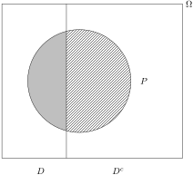
Observation: \(\Omega = D \cup D^c\text{,}\) so \(P = (P\cap D) \cup (P\cap D^c)\text{.}\)
Figure 29.
Observation 2:
\begin{align*} \Pr(P \mid D) \amp \frac{\Pr(P\cap D)}{\Pr(D)} \amp \amp \Rightarrow \amp \Pr(P \cap D) \amp = \Pr(P\mid D)\Pr(D) \\ \Pr(P \mid D^c) \amp \frac{\Pr(P\cap D^c)}{\Pr(D^c)} \amp \amp \Rightarrow \amp \Pr(P \cap D^c) \amp = \Pr(P\mid D^c)\Pr(D^c) \end{align*}
So:
\begin{gather*} \Pr(P) = \Pr(P\mid D)\Pr(D) + \Pr(P\mid D^c)\Pr(D^c) \end{gather*}
Example 31.
Continuing from the previous example:
\begin{align*} \Pr(D\mid P) \amp = \frac{\Pr(P\mid D)\Pr(D)}{\Pr(P\mid D)\Pr(D) + \Pr(P\mid D^c)\Pr(D^c)} \\ \amp = \frac{(0.9)(0.01)}{(0.9)(0.01) + (1 - 0.91)(1 - 0.01)} \\ \amp \approx 0.092 \end{align*}
What if the patient got a negative test result instead? In that case, what is the probaiblity they do not have the disease?
\begin{align*} \Pr(D^c\mid P^c) \amp = \frac{\Pr(P^c\mid D^c)\Pr(D^c)}{\Pr(P^c\mid D^c)\Pr(D^c) + \Pr(P^c\mid D)\Pr(D)} \\ \amp = \frac{(0.91)(1 - 0.01)}{(0.91)(1 - 0.01) + (1 - 0.9)(0.01)} \\ \amp \approx 0.999 \end{align*}

Subsubsection Independent Events

Question: \(\Pr(A \mid B)\) is supposed to capture how information about \(B\) affects the probability of \(A\text{.}\) What if it doesn’t?
Definition 32.
Events \(A, B\) are independent if \(\Pr(A \mid B) = \Pr(A)\text{.}\)
Observation: If \(A, B\) have nonzero probability and are independent, then:
\begin{align*} \Pr(A\mid B) \amp = \Pr(A) \\ \frac{\Pr(A\cap B)}{\Pr(B)} \amp = \Pr(A) \\ \Pr(A\cap B) \amp = \Pr(A)\Pr(B) \end{align*}
We can take this last equation as a definition of independence.
Example 33.
Continuing ExampleΒ 25, recall \(A = \{\text{sum} \geq 10\}\) and \(B = \{\text{1st roll is } 6\}\text{.}\) We found that \(\Pr(A \mid B) \neq \Pr(A)\text{,}\) so \(A\) and \(B\) are not independent.
Now consider the event \(C = \{\text{sum} = 7\}\text{.}\) We have:
\begin{align*} C \amp = \{(1, 6), (2, 5), (3, 4), (4, 3), (5, 2), (6, 1)\} \\ \Pr(C) \amp = \frac{6}{36} = \frac{1}{6} \\ B\cap C \amp = \{(6, 1)\} \\ \Pr(B\cap C) \amp = \frac{1}{36} \\ \text{therefore: } \Pr(C\mid B) \amp = \frac{\Pr(C\cap B)}{\Pr(B)} = \frac{1/36}{1/6} = \frac{1}{6} = \Pr(C) \end{align*}
Therefore events \(B, C\) are independent.